Methods Used by the Buzzards Bay NEP / MCZM Study of Flood Zone Expansion with Sea Level Rise
ArcMap GIS software (ArcView license) was used to manipulate the various existing digital data sets, with some additional analysis completed in spreadsheets using pivot table functions. No field collection of data or ground truthing was required for this analysis. We used a 2007 LiDAR study contracted by FEMA, and described in detail in CDM (2008). These LiDAR data were provided to the Buzzards Bay NEP as both 2-ft contour lines, and as digital elevation models (DEMs) in the form of Triangular Irregular Network (TIN) raster files. To a limited degree, for certain flood zone expansion areas we also used 2011 Northeast National Map LiDAR project data (unpublished). In general, the precision of the LiDAR data is 1 cm, but the accuracy is approximately 6 inches over the entire southeast study area, and the relative accuracy over a small geographic area along the same flight path is considerably better (USGS, 2004).
The base flood elevations from the Flood Insurance Rate Maps (FIRMs) released by FEMA for Fairhaven in 2009 were overlain on the detailed LiDAR contour data (Fig. 1) and digital elevation models (Fig. 2). Because the flood zone delineations on the FIRMs do not exactly follow LiDAR contours for a number of reasons, this step was necessary to establish a detailed baseline floodplain that could be consistently expanded by the projected sea level rise scenarios. Typically, the LiDAR 2-ft elevation contour lines were adequate to estimate expansion or adjustments of the boundaries each of the sea level rise scenario. However, where land slopes were slight, and the base flood elevation was set to an odd-number value, then TIN raster images were often used to visually estimate the respective new flood zone boundaries, as in Fig. 2. In this way a baseline floodplain zone was defined which was used as the initial conditions for the purposes of this study and allow for more meaningful and precise comparisons among the sea level rise scenarios.
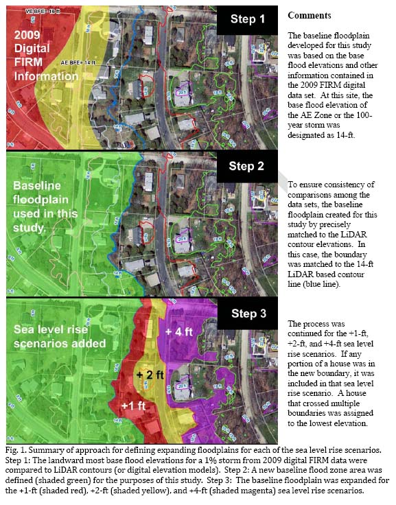
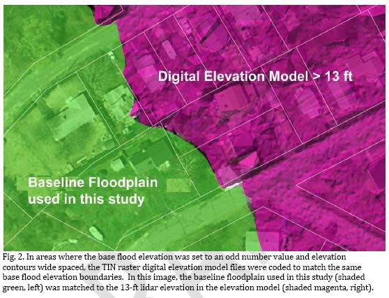
This baseline floodplain was then expanded to account for 1-, 2-, and 4-foot sea level rises by adjusting the boundaries to the LiDAR elevations that corresponded to the base flood elevations identified on the FIRMS (as in Figs. 1 and 2). Thus, if the base flood elevation on the FEMA FIRM was specified as 14 feet for a site, the boundary of the baseline floodplain would be expanded to the 18-ft LiDAR contour in the + 4-ft sea level rise scenario. This is a simplified approach, and a more accurate approach would have involved detailed engineering analyses to determine how much the flood elevations would rise along the coast given the submergence of land in the 0-4-ft zone, but such an effort was beyond the scope of this study.
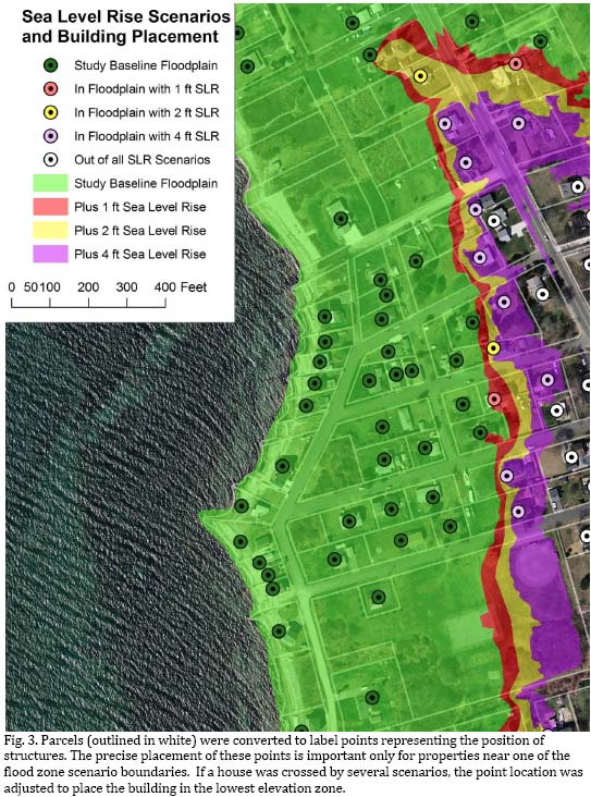
After the floodplain boundaries were created, assessor's data were applied to the GIS parcel data set. Because a building footprint coverage for Fairhaven was not available, centroid label points were created for each parcel to represent the location of each house. The position of these points was carefully examined along the boundary of each flood zone scenario and moved to coincide with the house footprint. If a house was crossed by several floodplain scenarios, the point, representing the vulnerability of the structure to sea level rise, was placed in the lowest elevation scenario as illustrated in Fig. 3 (note house near Indian Way). Secondary or ancillary detached structures were ignored, and the property building value was assigned to the main structure, typically the primary residential structure. On some parcels, there are multiple detached dwellings units, but no parcels of this particular type were bisected by a flood zone.
Once the position of structures was set relative to the sea level rise scenarios, and assigned assessed values for total building structures on the parcel linked to these points, this digital point coverage was intersected with flood zone sea level rise scenario polygons. The resulting data set was processed in an Excel spreadsheet, and a pivot table was used to quantify building data using various classifications of structures by flood zone and inside or outside of the hurricane barrier.
Work flow to address two or more tax records (typically of different owners) assigned to one parcel, and to assign the largest structure of multiple structures on assessor's parcels
Below are the workflow steps to create points associated with all tax records and to assign them to the location of the largest structure on the property. This work works well when a MassGIS Level 3 quality database is used.
The steps below are an exhaustive approach to minimize post processing and capture potential errors in the database by ensuring that all parcels have a point. This workflow will catch a small percentage of errors in the assessor's database, or where a structure is assigned to the wrong companion parcel. These types of errors can usually be found through visual evaluation of the coverage with appropriate labeling and color-coding of points and parcels, and by reviewing join counts.
A simplified workflow is possible using only ArcGIS, if a certain amount of potential errors (<1%) are acceptable). This alternate workflow is also described below. Further simplification can be made if only built parcels are evaluated.
At each step, consider deleting unnecessary generated fields to keep the database free of superfluous data. This workflow has some redundancy to prevent repeating steps in case of processing errors (e.g., accidentally deleting a vital field).
Steps
1) In ArcGIS, dissolve MassGIS parcels for LOC_ID.
2) In Geospatial Modeling Environment (Version 0.7.2.1), create X and Y label point coordinates for each parcel (function "genpointinpoly, " position label points, not centroids, copy all fields). This approach ensures that the point is inserted inside the parcel for odd shaped parcels. Create fields PXCOORD and PYCOORD with these values. These XY Coordinates will only be used for parcels that do not have building footprints.
Simple alternative: Create PXCOORD and PYCOORD in the parcel database and generate geometry centroids in the field calculator.
3) In ArcGIS, perform a spatial join of the MassGIS building footprint coverage for the respective town to the parcel coverage in step 1. In the spatial join function [arctoolbox > analysis tools > spatial join: target= structures, join features= parcel PXCOORD and PYCOORD file, join one-to-one], choose "have their center in" to assign the structure to the presumed correct parcel (this spatial join approach prevents splitting buildings and creating duplicate tax entries for the split buildings). The structures now all have a parcel LOC_ID assigned to them. Dissolved this coverage by LOC_ID (allow multipart). The new dissolved file will have multipart building structures with each parcel LOC_ID.
4) In Geospatial Modeling Environment (Version 0.7.2.1), create X and Y label point coordinates for each multipart structure (function "genpointinpoly, " label points, not centroids, are preferred, call the SXCOORD and SYCOORD) to ensure that the point is inserted inside a parcel (the software appears to default to the largest structure when multiple structures are present).
Simple alternative: Create SXCOORD and SYCOORD fields in the parcel database and generate geometry centroids in the field calculator.
5) In ArcGIS, perform a logical join of the structure point coverage to the parcel point coverages which include their respective PX, PY and SXCOORD and SYCOORD values using the common parcel LOC_ID field (keep all records, export to a new coverage). The resulting parcel point coverage has a building structure point coordinate for all parcels (SXCOORD, SYCOORD) with a building structure as well as the parcel label points (PX, PY). Create a new final coordinate field (FXCOORD and FYCOORD). First assign all PX, PY values to the FXCOORD FYCOORD, then for those with SXCOORD, SYCOORD values, assign the SXCOORD, SYCOORD values to the FXCOORD and FYCOORD fields. All points should now have the FXCOORD and FYCOORD with values, with the preference of structure coordinates if the structures exist. These FXCOORD and FYCOORD values can be assigned to the assessor's parcel coverage if needed using a logical join of the LOC_ID field.
8) In ArcGIS, open the MassGIS assessors database file (townTax.dbf) as a table. Join this table to the coverage with the FXCOORD and FYCOORD values. The resulting table now has the final xy coordinates, FXCOORD and FYCOORD, from step 7. Export to a new table name (e.g. M003_assess_fxfy).
9) Convert this table to a point coverage using the ArcGIS add FXCOORD FYCOORD coordinates. Save the resulting coverage to a new file (e.g. Acush_struc_parc_pts_assessors.shp). For parcels with structures, a point will be located in the largest structure; for parcels without a structure, the point will be located near the center of the parcel.
10) The point coverage in step 9 can be intersected with various flood zone and sea level rise scenarios.
Note certain steps could be omitted, and just the centroid feature of ArcGIS used, but there is a danger of some parcel structure values lost. These will likely total less than a fraction of 1% unless a large structure (e.g., a school) was assigned to wrong parcel and dropped out of the analysis, although visual inspections of the maps would generally catch such blatant omissions.
Method variations
We subsequently streamlined some of our data processing to reduce manual manipulation of moving points for structures bisected by multiple. In this alternative approach, before step 4 is taken, the following actions can be implemented to assign a flood zone scenario for each structure. These steps are as follows:
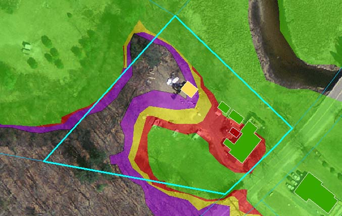
4A) Create a separate coverage for each floodplain SLR scenario. Add a field to the structure database called "SLR_SCEN." First, fill all records with the value "Out." Perform a "select by location" for each coverage, beginning with the highest SLR scenario (+4 ft in this case). With this first select by location, assign a value "SLR_SCEN"='BFE +4 ft'. Repeat this step for the other SLR scenarios. By selecting in reverse order, for those structures crossing multiple scenarios, the lowest flood zone scenario is selected. The graphic below shows the results on a parcel with 4 structures. Note that each structure is assigned to the lowest SLR_SCEN value it touches (in this case the color codes are green red yellow purple for the +0, +1, +2, +4 ft scenarios).
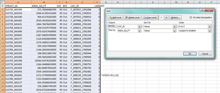
4B) The next step is to select out only the largest structure on each parcel. This step could have been done first, but in step 4A we wanted to demonstrate how all structures in an area be classified by intersection with multiple scenarios. To find the largest structure on each parcel you could either use the ArcGIS Date Review extension (which we do not), develop some SQL code (not always pleasant), or use the handy sort feature in a spreadsheet. We chose the latter as it was most expedition. This involves opening the shapefile dbf file in excel, deleting the unnecessary fields, then sorting first by Loc_ID (the parcel identifier, then by structure footprint area (largest to smallest see image below). A simple test by the formula shown in column E accurately identifies the largest structure on every parcel (parcels with only 1 structure are of course the larges. This spreadsheet is then exported as a CSV file (especially if there are more than 65k records), and joined back in the database by structure ID.
References
CDM-Smith, 2008. Flood Mapping Activities for Plymouth and Bristol Counties, Massachusetts (29 MB). Task Order 18 Activity 1--Topographic Data Development / Acquisition Summary Report. Contract No. EME-2003-CO-0340 Task Order T018. Prepared for: FEMA Region I, February 2008.
EEA (Massachusetts Executive Office of Energy and Environmental Affairs), 2011. Massachusetts Climate Change Adaptation Report September 2011. 128 pp. Available at http://www.mass.gov/eea/air-water-climate-change/climate-change/climate-change-adaptation-report.html.
Flood Insurance Management Agency (FEMA). 2003. Guidelines and Specifications for Flood Hazard Mapping Partners, Volume 1: Flood Studies and Mapping. 110 pp.
IPCC (Intergovernmental Panel on Climate Change), 2007. Climate Change 2007: The Physical Science Basis. Contribution of Working Group I to the Fourth Assessment Report of the Intergovernmental Panel on Climate Change [Solomon, S., D. Qin, M. Manning, Z. Chen, M. Marquis, K. B. Avery, M. Tignor, and H. L. Miller (eds.)]. Cambridge University Press, Cambridge, UK, and New York, 996 pp.
Risk Management Solutions, Inc. (RMSI), 2008. The 1938 Great New England Hurricane. Looking to the Past to Understand Today�s Risk. 23 pp.
USGS, 2004. Guidelines for Digital Elevation Data, Version 1.0, National Digital Elevation Program (NDEP), May 10, 2004 available at: http://www.ndep.gov/NDEP_Elevation_Guidelines_Ver1_10May2004.pdf
